Introduction¶

Here is a practical use of ROpenFLUID package for simulations and model analyses.
It is illustrated on the MHYDAS model (see notes for more details about the model and installation). The MHYDAS model is applied on a virtual catchment composed of 9 spatial units : 6 parcels (SUs) and 3 ditches (RSs) (see figure 1).

Figure 1: Spatial domain on which is applied MHYDAS model

This model represents and couples three processes (production function : separation of the rain into runoff and infiltration, water transfers on the SUs surface and water transfers in the RSs). The computed variables are :

• the infiltration and runoff height on the SUs,

• the flow rate at the outlet of the SUs and RSs,

• the water level on the RSs.

The model input factors which will be analysed are :

• the wave mean celerity on SUs,

• the wave mean celerity on RSs,

• the wave mean diffusivity on SUs and RSs,

• the initial water content on SUs,

• the saturated hydraulic conductivity on SUs.

Among the output variables, some of them characterize the global behaviour of the model (i.e. the flow rate at the outlet of the RS3, the global outlet of the virtual subcatchment), others characterize its local behaviour (i.e. the infiltration on each SUs). The three first input factors are parameters of the transfer models, the next two factors depend on the spatial units characteristics and control the runoff production. The others model factors: simulator parameters, spatial attributes and the rain height on each SUs (the input spatial and temporal variable) will not be analyzed in this example. The analysis of a such spatialized model should take into account the effects of the input factors on the output variables at the global and the local scale.

The following lines propose some examples of model analysis. Thanks to the ROpenFLUID package, simple simulations and model analysis are performed. The sensitivity and optimx R packages are used to perform expert analysis. Other R packages are required in the following script for rendering results (ggplot2) or for factors sampling (lhs). The input dataset can be found here as a zip file and the final R script can be download here.

A proposed approach to set factors, run a single simulation and access to results¶

1. Setting and running the simulation with the defaults factors:

• Preparing the simulation

library("ROpenFLUID")

inputDir  <- "path/to/MHYDAS/dataset"
outputDir <- "path/to/MHYDAS/outputs"

ofsim <- OpenFLUID.openDataset(inputDir)
OpenFLUID.setCurrentOutputDir(outputDir)
OpenFLUID.addVariablesExportAsCSV(ofsim, "RS", 3) # export all variables on the unit "RS#3"
OpenFLUID.addVariablesExportAsCSV(ofsim, "SU") # export all variables of class "SU"
# get default time step
dT <- OpenFLUID.getDefaultDeltaT(ofsim)

• Running the simulation with the default factors of the dataset

OpenFLUID.runSimulation(ofsim)

2. Defining structures and functions to simplify the input factors and output results management:

• Defining a structure to map the input factors of the MHYDAS model. The simulator parameters and spatial attributes are read "by batch" with dedicated ROpenFLUID commands and store in several synthetic lists. See the Manuals section for more details on these "by batch" commands.

simIDs    <- OpenFLUID.getSimulatorsIDs(ofsim)
simParams <- list()
for (simID in simIDs) {
    simParamNames      <- OpenFLUID.getSimulatorParamNames(ofsim, simID)
    simParams[[simID]] <- OpenFLUID.getSimulatorParams(ofsim, simID, simParamNames)
}
attrNames <- list()
attrs     <- list()
for (unitclass in OpenFLUID.getUnitsClasses(ofsim)) {
    attrNames[[unitclass]] <- OpenFLUID.getAttributesNames(ofsim, unitclass)
    IDs                    <- OpenFLUID.getUnitsIDs(ofsim, unitclass)
    attrs[[unitclass]]     <- OpenFLUID.getAttributes(ofsim, unitclass, IDs, attrNames[[unitclass]])
}
# display model factors mapping
cat("\nSIMULATORS PARAMETERS:")
for (simID in simIDs) {
    cat("\n-", simID, ":", paste(simParamNames, collapse = ", "))
}
cat("\nSPATIALIZED ATTRIBUTES:")
for (unitclass in OpenFLUID.getUnitsClasses(ofsim)) {
    cat("\n-", unitclass, ":", paste(attrNames[[unitclass]], collapse = ", "))
}

# set factor names to analyzed and their defaut values
factorNames <- c(
    "cellSU",
    "cellRS",
    "sigma",
    paste("thi", (1:6), sep = "_"),
    paste("Ks", (1:6), sep = "_")
)
nFactor   <- length(factorNames)
factorVal <- rep(NULL, times = nFactor)

factorVal[1] <- as.numeric(simParams[[simIDs[3]]][1, c("meancel")])
factorVal[2] <- as.numeric(simParams[[simIDs[4]]][1, c("meancel")])
factorVal[3] <- as.numeric(simParams[[simIDs[4]]][1, c("meansigma")])
# /!\ thetaini is bounded by thetares and thetasat, the analyzed factor is the relative initial humidity
factorVal[4:9] <- (as.numeric(attrs[["SU"]][, "thetaini"]) - as.numeric(attrs[["SU"]][, "thetares"])) /
    (as.numeric(attrs[["SU"]][, "thetasat"]) - as.numeric(attrs[["SU"]][, "thetares"]))
factorVal[10:15] <- as.numeric(attrs[["SU"]][, "Ks"])

• Defining a generic function to gather an output variables set in a synthetic list

#
# ofsim      : the simulation definition
# unitclass  : the unit class name
# OFnames    : a vector of OpenFLUID variable names of the class unitclass
# shortnames : a vector of short variables names used as return list headings
# out        : an existing list obtains with this function
# 
# return     : a list gathering the variable values
#
getSpatialResults <- function(
    ofsim, unitclass, unitids, OFnames, shortnames, out = NULL
) {

    for (varname in OFnames) {
        shortname <- shortnames[which(varname == OFnames)]
        for (ID in unitids) {
            var <- OpenFLUID.loadResult(ofsim, unitclass, ID, varname)
            colheader <- paste(unitclass, ID, shortname, sep = "")
            if (is.null(out)) {
                out <- var
                colnames(out) <- c("datetime", colheader)
            } else {
                stopifnot(var[, 1] == out[, "datetime"])
                stopifnot(!(colheader %in% colnames(out)))
                out <- cbind(out, var[, 2])
                colnames(out) <- c(colnames(out)[1:(ncol(out) - 1)], colheader)
            }
        }
    }
    return(out)
}

• Defining a specific function to gather the selected variables set of a MHYDAS simulation in a synthetic list

#
# ofsim  : the simulation definition
# 
# return : a list gathering the following variables set :
#              ** global     : common datetime for all variables (datetime)
#              ** on all SUs : rain (SUxxRR), infiltration (SUxxI) and discharge rate (SUxxQ)
#              ** on RS3     : discharge rate (RS3Q)
#
getSelectedSimResults <- function(ofsim) {

    out <- getSpatialResults(
        ofsim,
        "SU",
        OpenFLUID.getUnitsIDs(ofsim, "SU"),
        c("water.atm-surf.H.rain", "water.surf.H.infiltration", "water.surf.Q.downstream-su"),
        c("RR", "I", "Q")
    )
    out <- getSpatialResults(
        ofsim,
        "RS",
        c(3),
        c("water.surf.Q.downstream-rs"),
        c("Q"),
        out
    )
    return(out)
}

• Evaluating aggregated indicators on the simulation

#
# ofsim       : the simulation definition
# outProvided : a list obtained with previous function
# return      : a list gathering the following indicators :
#               ** on SU5 : cumulative rain, infiltrated and exported volume (sumSU5RR,sumSU5I,sumSU5V) and time transfer (tmaxSU5Q)
#               ** on RS3 : the same indicator for the whole subcatchment (sumSURR,sumSUI,sumRS3V,tmaxRS3Q)
#
aggregateSelectedSimResults <- function(ofsim, outProvided = NULL) {

    if (is.null(outProvided)) {
        out <- getSelectedSimResults(ofsim)
    } else {
        out <- outProvided
    }

    # simulation default time step
    dT <- OpenFLUID.getDefaultDeltaT(ofsim)
    # cumulative rain, infiltration and runoff in SU5 (spatialized outputs)
    SU5Area <- as.numeric(as.numeric(attrs[["SU"]]$area[5]))
    SU5RR   <- sum(out$SU5RR) * SU5Area
    SU5I    <- sum(out$SU5I) * SU5Area
    SU5V    <- sum(out$SU5Q) * dT
    # time for maximum water discharge at the SU#5 outlet (spatialized output)
    if (max(out$SU5Q) > 0) {
        SU5TMax <- as.numeric(
            difftime(
                out$datetime[which.max(out$SU5Q)],
                out$datetime[which.max(out$SU5RR)],
                units = "hour"
            )
        )
    } else {
        SU5TMax <- NA
    }
    # cumulative rain and infiltration in the whole catchment (global outputs)
    SURR <- 0
    SUI  <- 0
    for (SUID in OpenFLUID.getUnitsIDs(ofsim, "SU")) {
        SUArea <- as.numeric(as.numeric(attrs[["SU"]]$area[SUID]))
        SURR   <- SURR + sum(out[, paste("SU", SUID, "RR", sep = "")]) * SUArea
        SUI    <- SUI  + sum(out[, paste("SU", SUID, "I", sep = "")]) * SUArea
    }
    # cumulative water volume at the subcatchment outlet (global output)
    RS3V <- sum(out$RS3Q) * dT
    # time for maximum water discharge at the subcatchment outlet (global output)
    if (max(out$RS3Q) > 0) {
        RS3TMax <- as.numeric(
            difftime(
                out$datetime[which.max(out$RS3Q)],
                out$datetime[which.max(out$SU5RR)],
                units = "hour"
            )
        )
    } else {
        RS3TMax < -NA
    }

    # return aggregated results as list
    return(
        data.frame(
            "sumSU5RR" = SU5RR,
            "sumSU5I"  = SU5I,
            "sumSU5V"  = SU5V,
            "tmaxSU5Q" = SU5TMax,
            "sumSURR"  = SURR,
            "sumSUI"   = SUI,
            "sumRS3V"  = RS3V,
            "tmaxRS3Q" = RS3TMax
        )
    )
}

• Defining a function to run a single simulation with modified factors

#
# ofsim    : the simulation definition
# X[1]     : simulator parameter meancelSU -> simParams[[ simIDs[3] ]]
# X[2]     : simulator parameter meancelRS -> simParams[[ simIDs[4] ]]
# X[3]     : simulator parameter meansigma -> simParams[[ simIDs[3] ]] and simParams[[ simIDs[4] ]]
# X[4:9]   : spatialized attributes thetaini -> attrs[["SU"]][,"thetaini"]
# X[10:15] : spatialized attributes Ks -> attrs[["SU"]][,"Ks"]
#
# return   : a list containing all the output variables and the aggregated results
#
runOneSim <- function(X, ofsim) {
    # set parameters for simulator : water.surf.transfer-su.hayami
    simParams[[simIDs[3]]][1, c("meancel", "meansigma")] <- c(X[1], X[3])
    OpenFLUID.setSimulatorParams(ofsim, simIDs[3], simParams[[simIDs[3]]])
    # set parameters for simulator : water.surf.transfer-rs.hayami
    simParams[[simIDs[4]]][1, c("meancel", "meansigma")] <- c(X[2], X[3])
    OpenFLUID.setSimulatorParams(ofsim, simIDs[4], simParams[[simIDs[4]]])
    # set attributes for class "SU"
    thetares <- as.numeric(attrs[["SU"]][, "thetares"])
    thetasat <- as.numeric(attrs[["SU"]][, "thetasat"])
    attrs[["SU"]][, "thetaini"] <- thetares + X[4:9] * (thetasat - thetares)
    attrs[["SU"]][, "Ks"]       <- X[10:15]
    OpenFLUID.setAttributes(ofsim, "SU", attrs[["SU"]])
    OpenFLUID.runSimulation(ofsim)
    out <- getSelectedSimResults(ofsim)
    return(
        list(
            "byTimeStep" = out,
            "indicators" = aggregateSelectedSimResults(ofsim, out)
        )
    )

}

3. Rendering the first results:

• Checking the surface water mass balance : rain is equal to infiltrated water added to exported water

# running MHYDAS simulation with default factors values
out <- runOneSim(factorVal, ofsim)
aggInd <- aggregateSelectedSimResults(ofsim, out$byTimeStep)
cat("\nCheck water mass balance on SU5 : ")
cat("\n - cumulative rain volume        :", aggInd$sumSU5RR)
cat("\n - cumulative infiltrated volume :", aggInd$sumSU5I)
cat("\n - cumulative exported volume    :", aggInd$sumSU5V)
cat(
    "\n - mass balance error            :",
    aggInd$sumSU5RR - (aggInd$sumSU5I + aggInd$sumSU5V)
)
cat("\nCheck water mass balance on subcatchment : ")
cat("\n - cumulative rain volume        :", aggInd$sumSURR)
cat("\n - cumulative infiltrated volume :", aggInd$sumSUI)
cat("\n - cumulative exported volume    :", aggInd$sumRS3V)
cat(
    "\n - mass balance error            :",
    aggInd$sumSURR - (aggInd$sumSUI + aggInd$sumRS3V)
)
cat("\n")

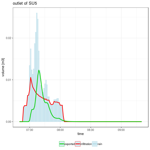
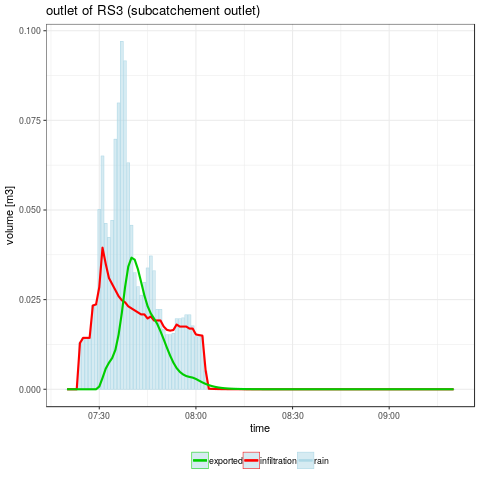
• Plotting the temporal evolution of the selected variables

library("ggplot2")

#
# ofsim       : the simulation definition blob
# outProvided : a list of results obtained with the previous functions
# return      : a list of ggplot
#
plotSimResults <- function(ofsim, outProvided = NULL) {

    dT  <- OpenFLUID.getDefaultDeltaT(ofsim)
    if (is.null(outProvided)) {
        out <- getSelectedSimResults(ofsim)
    } else {
        out <- outProvided
    }

    # cumulative rain and infiltration in the whole catchment (global output)
    SUArea <- as.numeric(attrs[["SU"]]$area)
    SURR   <- rep(0, length(out$datetime))
    SUI    <- SURR
    for (SUID in OpenFLUID.getUnitsIDs(ofsim, "SU")) {
        SURR   <- SURR + out[, paste("SU", SUID, "RR", sep = "")] * SUArea[SUID]
        SUI    <- SUI  + out[, paste("SU", SUID, "I", sep = "")] * SUArea[SUID]
    }
    out <- cbind(out, "SURR" = SURR)
    out <- cbind(out, "SUI" = SUI)
    # water volume exported at the subcatchment outlet
    out <- cbind(out, "RS3V" = out$RS3Q * dT) # from discharge to volume

    # cumulative rain, infiltration and water volume exported at the SU5 outlet, (spatialized output)
    SU5Area   <- as.numeric(as.numeric(attrs[["SU"]]$area[5]))
    out$SU5RR <- out$SU5RR * SU5Area # from height to volume
    out$SU5I  <- out$SU5I * SU5Area # from height to volume
    out       <- cbind(out, "SU5V" = out$SU5Q * dT) # from discharge to volume

    colors <- c("rain" = "lightblue", "infiltration" = "red", "exported" = "green3")
    # plot results on the unit "SU#5", spatialized outputs
    gpSU5 <- ggplot(out, aes(x = datetime)) + theme_bw() +
        geom_bar(
            aes(y = SU5RR, color = "rain"),
            fill  = "lightblue",
            stat  = "identity",
            alpha = .5,
            size  = 0.25
        ) +
        geom_line(aes(y = SU5I, color = "infiltration"), size = 1) +
        geom_line(aes(y = SU5V, color = "exported"), size = 1) +
        labs(
            title = "outlet of SU5",
            x     = "time",
            y     = "volume [m3]",
            color = ""
        ) +
        scale_color_manual(values = colors) +
        theme(legend.title = element_blank()) +
        theme(legend.position = "bottom")

    # plot aggregated results on the subcatchement, global outputs
    gpRS3 <- ggplot(out, aes(x = datetime)) + theme_bw() +
        geom_bar(
            aes(y = SURR,
            color = "rain"),
            fill  = "lightblue",
            stat  = "identity",
            alpha = .5,
            size  = 0.25
        ) +
        geom_line(aes(y = SUI, color = "infiltration"), size = 1) +
        geom_line(aes(y = RS3V, color = "exported"), size = 1) +
        labs(
            title = "outlet of RS3 (subcatchement outlet)",
            x     = "time",
            y     = "volume [m3]",
            color = ""
        ) +
        scale_color_manual(values = colors) + 
        theme(legend.title = element_blank()) +
        theme(legend.position = "bottom")
    return(list(SU5 = gpSU5, RS3 = gpRS3))

}
# plot results
gpRes <- plotSimResults(ofsim, out$byTimeStep)
png("graphics/resultsSU5.png")    
gpRes$SU5
dev.off()
png("graphics/resultsRS3.png")    
gpRes$RS3
dev.off()

Figure 2: cumulative rain, infiltrated and exported water heights on SU5 (left) and volumes on the whole subcatchment (right) (warning: Y axis have not the same scale for both graphics)

Some elements for model's behaviour analysis¶

(from here, random samplings can be used, the results you will get may be different from the results presented above)

1. Get the design of experiments and the model responses:

• Defining the factors boundaries: values have been choosen to have a non null exported water volume at the outlet of the subcatchment for the most of the simulations.

factorMin <- rep(NA, nFactor)
factorMax <- rep(NA, nFactor)

# cellSU: should not exceed flowdist/dT
factorMin[1] <- 1e-3
factorMax[1] <- 0.9 * min(as.numeric(attrs[["SU"]][, "flowdist"])) / dT
# cellRS: should not exceed length/dT
factorMin[2] <- 2.5e-3
factorMax[2] <- 0.9 * min(as.numeric(attrs[["RS"]][, "length"])) / dT
# cellSigma
factorMin[3] <- 100
factorMax[3] <- 2000
#thi: from moderate dry to saturated initial water content
factorMin[4:9] <- 0.33
factorMax[4:9] <- 0.99
#Ks: from high (clay soils) to moderate (loam soils) impermeability
factorMin[10:15] <- 1e-7
factorMax[10:15] <- 1e-5

• Defining a design of experiments (Sobol2002 from sensitivity package) to explore model responses

library("lhs")
library("sensitivity")

#
# nSlice, nRepeat : slices and repeats numbers
# XMin, XMax      : the factors boundaries
# factorNames    : a vector of the factor names
#
# return : a list of two factors sampling (X1, X2)
#
generateSobolRandomSamples <- function(nSlice, nRepeat, XMin, XMax, factorNames) {

    set.seed(123)

    nFactors <- length(factorNames)
    X1 <- NULL
    for (i in 1:nRepeat) {
        ech    <- randomLHS(nSlice, nFactors)
        for (j in 1:nFactors) {
            ech[, j] <- XMin[j] + ech[, j] * (XMax[j] - XMin[j])
        }
        X1 <- rbind(X1, ech)
    }
    X2 <- NULL
    for (i in 1:nRepeat) {
        ech    <- randomLHS(nSlice, nFactors)
        for (j in 1:nFactors) {
            ech[, j] <- XMin[j] + ech[, j] * (XMax[j] - XMin[j])
        }
        X2 <- rbind(X2, ech)
    }
    X1 <- as.data.frame(X1)
    names(X1) <- factorNames
    X2 <- as.data.frame(X2)
    names(X2) <- factorNames
    return(list(X1 = X1, X2 = X2))

}

nSlice       <- 50
nRepeat      <- 25
SobolSamples <- generateSobolRandomSamples(
    nSlice,
    nRepeat,
    factorMin,
    factorMax,
    factorNames
)
DOE <- sobol2002(
    model = NULL,
    X1    = SobolSamples$X1,
    X2    = SobolSamples$X2,
    conf  = 0.95,
    nboot = 100
)
NSimu <- dim(DOE$X)[1]

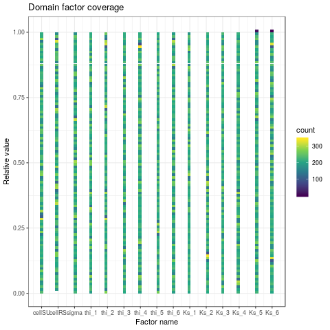
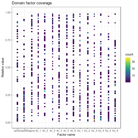
• Checking the coverage of the factors domain

#
# DOE    : the design of experiments (data.frame)
#
# return : a ggplot
#
plotDOECoverage <- function(DOE) {

    DOECov <- data.frame()
    for (i in 1:nFactor) {
        relval <- (DOE[, i] - factorMin[i]) / (factorMax[i] - factorMin[i])
        DOECov <- rbind(DOECov, data.frame("name" = i - 0.9, "relval" = relval))
    }

    return(
        ggplot(DOECov, aes(x = name, y = relval)) +
            ggtitle("Domain factor coverage") +
            xlab("Factor name") + ylab("Relative value") + ylim(0, 1) +
            scale_x_continuous(breaks = (1:nFactor) - 0.9, labels = factorNames) +
            theme(axis.text.x = element_text(angle = 90, hjust = 1)) +
            geom_bin2d(bins = c(5 * nFactor, 100)) +
            theme_bw() + scale_fill_continuous(type  =  "viridis")
    )
}
png("graphics/DOECoverage.png")
plotDOECoverage(DOE$X)
dev.off()

Figure 3: The factors domain coverage of the computed design of experiments

• Running a set of simulations at once and return the model responses as a list

#
# ofsim  : the simulation definition
# X      : the matrix of factors (NSimu x NFactors)
#
# return : a list containing all the output variables and the aggregated results
#
runMultiSim <- function(X, ofsim) {

    NSimu <- dim(X)[1]
    outIndicators <- data.frame()
    outByTimeStep <- list()
    cat("\nRUN ", NSimu, " SIMULATIONS:")
    cat("\n")
    for (i in rownames(X)) {
        # display run progress
        nInProgress <- floor(20 * as.numeric(i) / NSimu)
        cat(
            "\rsimulations in progress ",
            rep("o", nInProgress),
            rep("-", (20 - nInProgress)),
            " [", i, "/", NSimu, "]",
            sep = ""
        )
        # run current simulation
        runOneSim(as.numeric(X[i, ]), ofsim)
        # get and store results
        out <- getSelectedSimResults(ofsim)
        outByTimeStep[[paste("simu", i, sep = "")]] <- out
        outIndicators <- rbind(
            outIndicators,
            aggregateSelectedSimResults(ofsim, out)
        )
    }
    cat("\nall ", NSimu, "simulations done.\n")
    return(
        list(
            "indicators" = outIndicators,
            "byTimeStep" = outByTimeStep
        )
    )

}

# run the N simulations and get the model responses
# /!\ may take some time (0.1s / simulations on a Intel(R) Xeon(R) CPU E5-2609 v4 @ 1.70GHz)
Y <- runMultiSim(DOE$X, ofsim)
X <- DOE

• Saving design of experiments and model responses for further analysis

save(list = c("X", "Y"), file = "rdata/DOE-50-25.rdata")

• Reloading previously computed model responses: skip previous steps and run

load(file = "rdata/DOE-50-25.rdata")
NSimu <- dim(X$X)[1]

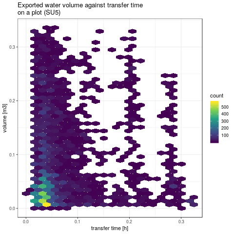
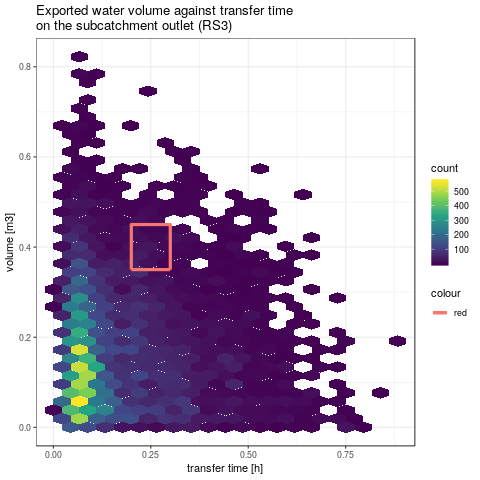
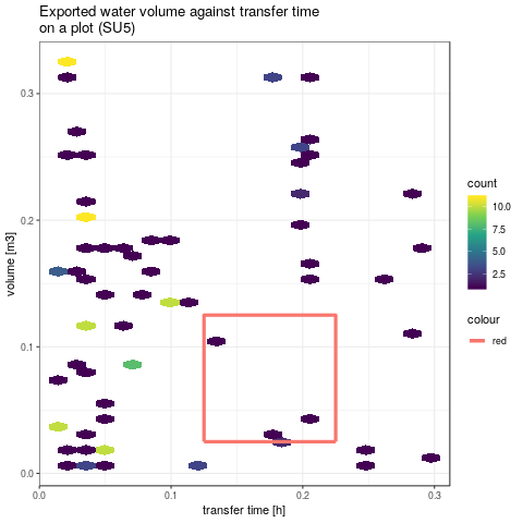
• Rendering some global results: plot water exported volume against transfer time for both SU5 and subcatchement

#
# YIndicators : aggregated indicators from model responses
# iToPlot     : simulation indexes to render in plot
#
# return      : a list of ggplot objects
#
plotVolTMax <- function(YIndicators, iToPlot, nbins) {

    iToPlotSU5 <- intersect(iToPlot, which(YIndicators$sumSU5V != 0))
    iToPlotRS3 <- intersect(iToPlot, which(YIndicators$sumRS3V != 0))

    YVolTMaxSU5 <- data.frame(
        x = YIndicators$tmaxSU5Q[iToPlotSU5],
        y = YIndicators$sumSU5V[iToPlotSU5]
    )
    YVolTMaxRS3 <- data.frame(
        x = YIndicators$tmaxRS3Q[iToPlotRS3],
        y = YIndicators$sumRS3V[iToPlotRS3]
    )

    gpSU5 <- ggplot() +
        geom_hex(data = YVolTMaxSU5, aes(x = x, y = y), bins = nbins) + theme_bw() + 
        scale_fill_continuous(type = "viridis") +
        ggtitle("Exported water volume against transfer time\non a plot (SU5)") + 
        xlab("transfer time [h]") + ylab("volume [m3]")
    gpRS3 <- ggplot() +
        geom_hex(data = YVolTMaxRS3, aes(x = x, y = y), bins = nbins) + theme_bw() + 
        scale_fill_continuous(type = "viridis") +
        ggtitle("Exported water volume against transfer time\non the subcatchment outlet (RS3)") + 
        xlab("transfer time [h]") + ylab("volume [m3]")

    return(list("SU5" = gpSU5, "RS3" = gpRS3))

}
gpVolTMax <- plotVolTMax(Y$indicators, 1:NSimu, c(20, 40))
png(paste(RDir, "graphics/vol2tmaxSU5.png", sep = "/"))
gpVolTMax$SU5
dev.off()
png(paste(RDir, "graphics/vol2tmaxRS3.png", sep = "/"))
gpVolTMax$RS3
dev.off()

Figure 4: exported water volume against transfer time on SU5 (left) and on the whole subcatchment (right)

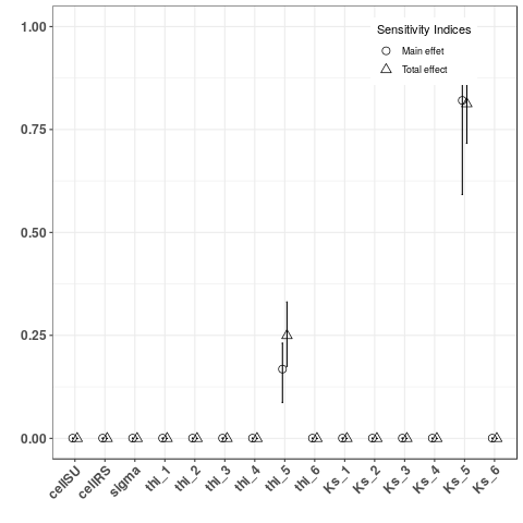
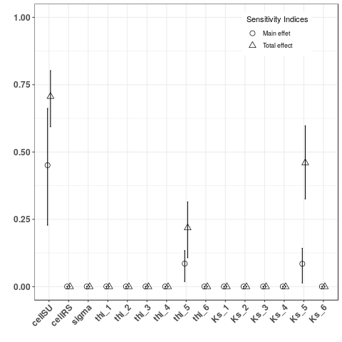
2. Sobol indices of two kind of output:

• Computed and plot Sobol indices on indicators sumSU5V and tmaxSU5Q, two local indicators

YVSU5 <- Y$indicators$sumSU5V
tell(X, YVSU5)
png("graphics/sobolSU5V.png")
ggplot(X)
dev.off()

YTMaxSU5 <- Y$indicators$tmaxSU5Q
iTMaxNASU5 <- which(is.na(YTMaxSU5))
# /!\ if the volume exported is null, transfer time is NA, replace them by 0
YTMaxSU5[iTMaxNASU5] <- 0
tell(X, YTMaxSU5)
png("graphics/sobolSU5TMax.png")
ggplot(X)
dev.off()

Figure 3a: Sobol indices for the exported water volume on SU5 (left) and for the transfer time (right): as expected, results are only influenced by global parameters and local attrbutes. The sensitivity on the exported volume is only due to initial humidity and hydraulic conductivity of the SU5, the transfer time is also sensitive to the mean wave celerity on SU.

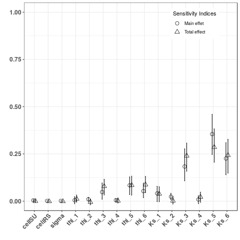
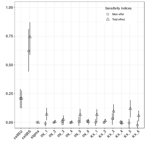
• Computed and plot Sobol indices on indicators sumRS3V and tmaxRS3Q, two global indicators

YV <- Y$indicators$sumRS3V
tell(X, YV)
png("graphics/sobolRS3V.png")
ggplot(X)
dev.off()

YTMax <- Y$indicators$tmaxRS3Q
# /!\ if the volume exported is null, transfer time is NA, replace them by 0
iTMaxNA <- which(is.na(YTMax))
YTMax[iTMaxNA] <- 0
tell(X, YTMax)
png("graphics/sobolRS3TMax.png")
ggplot(X)
dev.off()

Figure 3b: Sobol indices for the exported water volume on RS3 (left) and for the transfer time (right): the exported water volume is mainly due to runoff production, especially these of nearest SUs from outlet, thereas the time transfer is mainly due to the mean wave celerity.

Some elements for model's calibration¶

1. Calibration with observations on cumulative volume and transfer time at global scale:

• Let's consider the cumulative volume and the transfer time have been measured at the outlet of subcatchment (respectively 0.25m3 and 0.4h with an arbitrary measure error of 0.05m3 and 0.05h). We try first to identify the factors sets leading to these model responses.

# define a bounding box centered at 0.25 +/- 0.05 and 0.4 +/- 0.05
boxCenter   <- c(0.25, 0.4)
boxSize     <- c(0.1, 0.1)
boundingBox <- data.frame(
    "x" = (boxCenter[1] - 0.5 * boxSize[1]),
    "y" = (boxCenter[2] - 0.5 * boxSize[2])
)
boundingBox <- rbind(
    boundingBox,
    data.frame(
        "x" = (boxCenter[1] - 0.5 * boxSize[1]),
        "y" = (boxCenter[2] + 0.5 * boxSize[2])
    )
)
boundingBox <- rbind(
    boundingBox,
    data.frame(
        "x" = (boxCenter[1] + 0.5 * boxSize[1]),
        "y" = (boxCenter[2] + 0.5 * boxSize[2])
    )
)
boundingBox <- rbind(
    boundingBox,
    data.frame(
        "x" = (boxCenter[1] + 0.5 * boxSize[1]),
        "y" = (boxCenter[2] - 0.5 * boxSize[2])
    )
)
boundingBox <- rbind(
    boundingBox,
    data.frame(
        "x" = (boxCenter[1] - 0.5 * boxSize[1]),
        "y" = (boxCenter[2] - 0.5 * boxSize[2])
    )
)

# drawing this bounding box on the model responses graphics
png(paste(RDir, "graphics/vol2tmaxRS3-withBox.png", sep = "/"))
gpVolTMax$RS3 + 
    geom_line(data = boundingBox[1:4, ], aes(x = x, y = y, color = "red"), size = 1.5) +
    geom_line(data = boundingBox[4:5, ], aes(x = x, y = y, color = "red"), size = 1.5)
dev.off()

# drawing factors domain coverage
iMatchBox <- intersect(
    which(
        (Y$indicators$tmaxRS3Q > boundingBox[1, 1]) &
        (Y$indicators$tmaxRS3Q < boundingBox[3, 1])
    ),
    which(
        (Y$indicators$sumRS3V > boundingBox[1, 2]) &
        (Y$indicators$sumRS3V < boundingBox[3, 2])
    )
)
png(paste(RDir, "graphics/DOECoverage-withBox.png", sep = "/"))
plotDOECoverage(X$X[iMatchBox, ])
dev.off()

Figure 4: Model responses at RS3 (left) and factor domain coverage leading to the measured cumulative volume and transfer time at the outlet of virtual subcatchment (right). A problem of equifinality is obvious here: several set of factors lead to the same model response. For instance, 2 simulations with an high infiltrability on only SU3 or SU5, all other infilitrabilities set to a very low value, could lead to the same cumulative volume. In the first case, exported water at outlet will be due only to SU3 runoff, in the second case to SU5. Without complementary measures or other data (i.e. expert opinions), model calibration will be impossible.

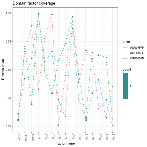
2. Calibration with observations on cumulative volume and transfer time at local and global scale:

• Let's now consider the same quantities have been also monitored at the outlet of SU5 (respectively 0.175m3 and 0.075h with the same measure error). Among the previously selected factors sets in the last analysis, the same screening is performed based on the model responses on SU5.

# define a bounding box centered at 0.175 +/- 0.05 and 0.075 +/- 0.05
boxCenterSU5   <- c(0.175, 0.075)
boundingBoxSU5 <- data.frame(
    "x" = (boxCenterSU5[1] - 0.5 * boxSize[1]),
    "y" = (boxCenterSU5[2] - 0.5 * boxSize[2])
)
boundingBoxSU5 <- rbind(
    boundingBoxSU5, data.frame(
        "x" = (boxCenterSU5[1] - 0.5 * boxSize[1]),
        "y" = (boxCenterSU5[2] + 0.5 * boxSize[2])
    )
)
boundingBoxSU5 <- rbind(
    boundingBoxSU5, data.frame(
        "x" = (boxCenterSU5[1] + 0.5 * boxSize[1]),
        "y" = (boxCenterSU5[2] + 0.5 * boxSize[2])
    )
)
boundingBoxSU5 <- rbind(
    boundingBoxSU5, data.frame(
        "x" = (boxCenterSU5[1] + 0.5 * boxSize[1]),
        "y" = (boxCenterSU5[2] - 0.5 * boxSize[2])
    )
)
boundingBoxSU5 <- rbind(
    boundingBoxSU5, data.frame(
        "x" = (boxCenterSU5[1] - 0.5 * boxSize[1]),
        "y" = (boxCenterSU5[2] - 0.5 * boxSize[2])
    )
)

# drawing this bounding box on the model responses graphics
gpVolTMaxWithBox <- plotVolTMax(Y$indicators, iMatchBox, c(20, 40))
png(paste(RDir, "graphics/vol2tmaxSU5-withBox.png", sep = "/"))
gpVolTMaxWithBox$SU5 +
    geom_line(
        data = boundingBoxSU5[1:4, ],
        aes(x = x, y = y, color = "red"),
        size = 1.5
    ) +
    geom_line(
        data = boundingBoxSU5[4:5, ],
        aes(x = x, y = y, color = "red"),
        size = 1.5
    )
dev.off()

# drawing factors domain coverage
iMatchBoxSU5 <- iMatchBox[intersect(
    which(
        (Y$indicators$tmaxSU5Q[iMatchBox] > boundingBoxSU5[1, 1]) &
        (Y$indicators$tmaxSU5Q[iMatchBox] < boundingBoxSU5[3, 1])
    ),
    which(
        (Y$indicators$sumSU5V[iMatchBox] > boundingBoxSU5[1, 2]) &
        (Y$indicators$sumSU5V[iMatchBox] < boundingBoxSU5[3, 2])
    )
)]

png(paste(RDir, "graphics/DOECoverage-withBoxSU5.png", sep = "/"))
gpFactors <- plotDOECoverage(X$X[iMatchBoxSU5, ])
for (i in 1:length(iMatchBoxSU5)) {
    name <- ((1:nFactor) - 0.9)
    relval <- as.numeric(
        (X$X[iMatchBoxSU5[i], ] - factorMin) / (factorMax - factorMin)
    )
    color  <- rainbow(length(iMatchBoxSU5))[i]
    gpFactors <- gpFactors +
        geom_line(
            data = data.frame(name, relval, color),
            aes(x = name, y = relval, color = color),
            size     = 0.5,
            linetype = "dashed"
        )
}
gpFactors
dev.off()

Figure 5: Model responses at SU5 (left) and factor domain coverage leading to the measured cumulative volume and transfer time at both the outlet of virtual subcatchment and SU5(right). The dashed lines connect the factors set. The number of matching simulations is drasticly reduced and the problem of equifinality is clearly reduced for some factors.

3. Automatic calibration with observations on cumulative volume and transfer time at local scale:

• Defining the objective function to optimize. For results on SU5, only mean cell on SU, initial humidity and hydraulic conductivity are sensitive.

# reduce factor domain 
factorMinReduc <- c(
    0,      # meancellSU
    0.25,   # meancellRS
    0,      # meansigma: not sensitive
    0.25,   # thi_1
    0,      # thi_2: not sensitive
    0.25,   # thi_3
    0,      # thi_4: not sensitive
    0,      # thi_5
    0.75,   # thi_6
    0,      # Ks_1
    0,      # Ks_2: not sensitive
    0.25,   # Ks_3
    0,      # Ks_4: not sensitive
    0,      # Ks_5
    0       # Ks_6
)
factorMaxReduc <- c(
    0.25,   # meancellSU
    0.75,   # meancellRS
    1,      # meansigma: not sensitive
    1,      # thi_1
    1,      # thi_2: not sensitive
    1,      # thi_3
    1,      # thi_4: not sensitive
    0.75,   # thi_5
    1,      # thi_6
    0.5,    # Ks_1
    1,      # Ks_2: not sensitive
    0.75,   # Ks_3
    1,      # Ks_4: not sensitive
    0.75,   # Ks_5
    0.5     # Ks_6
)
lower <- factorMin + factorMinReduc * (factorMax - factorMin)
upper <- factorMin + factorMaxReduc * (factorMax - factorMin)

iFactorSensitive <- c(1, 8, 14)

# define ojective function
ref          <- data.frame("tmaxSU5Q" = 0.175, "sumSU5V" = 0.075)
objectiveFct <- function(X, factorOther, ofsim, ref) {
    factorCurrent                   <- factorOther
    factorCurrent[iFactorSensitive] <- X
    out                             <- runOneSim(factorCurrent, ofsim)
    if (is.na(out$indicators$tmaxSU5Q)) {
        out$indicators$tmaxSU5Q <- 0
    }
    return(sum((out$indicators[c("tmaxSU5Q", "sumSU5V")] - ref)**2))
}

• Running automatic calibration with optimx R package, initial guess is one of the previous sets of factors, the choosen method is the Nelder-Mead algorithm for derivative-free optimization.

library("optimx")
X0 <- as.numeric(X$X[iMatchBoxSU5[1], iFactorSensitive])
objFct0 <- objectiveFct(X0, as.numeric(X$X[iMatchBoxSU5[1], ]), ofsim, ref)
factorOptim <- optimx(
    X0,
    fn          = objectiveFct,
    lower       = lower[iFactorSensitive],
    upper       = upper[iFactorSensitive],
    method      = "nmkb",
    factorOther = as.numeric(X$X[iMatchBoxSU5[1], ]),
    ofsim       = ofsim,
    ref         = ref
)
# replace method = "nmkb" by a vector of methods or by the argument control = list(all.methods = TRUE) to compare several methods
summary(factorOptim)

• The Nelder-Mead algorithm reduces the objective function from 0.0027 to 0.0001 and adjust the 3 sensitive factors.

> X0
[1] 9.435129e-03 3.835945e-01 8.358475e-07
> objFct0
[1] 0.002655506
> summary(factorOptim)
              p1        p2           p3        value fevals gevals niter
nmkb 0.006786553 0.5585314 1.416184e-06 0.0001007124    103     NA    NA
     convcode  kkt1  kkt2 xtime
nmkb        0 FALSE FALSE 8.246
>